Overview
What is SNARE?
SNARE is a modular audio analyze tool focused on handling long multichannel recordings. It includes a standardized octave band analysis, sound pressure level over time and histogram (sound pressure level occurrence distribution) with the option to calibrate analysis and generate reports. Analysis can be extended by a plugin system. It is implemented in Python, open source and cross-platform. SNARE can use 16bit or 24bit with 44.1kHz, 48kHz or 96kHz WAV files with an arbitrary number of channels as data source or directly record multiple channels from any audio interface. The tool supports a calibration source with 94dB at 1kHz otherwise it can perform quantitative analysis.
The first part of this thesis features a short tutorial on how-to use SNARE, a detailed manual describing all aspects of the tool, as well as a guide to extending the tool’s functionality, while the second part covers the development and technical documentation.
This is something I want to say that is not in the docstring.
User Manual
2.1 Quick Guide
2.1.1 Step 1: Select input
2.1.2 Step 2: Calibrate (optional)
2.1.3 Step 3: Analyse
2.1.4 Step 4: Export
2.2 User Manual
2.2.1 Data flow chart and layout
2.2.2 Open file(s)
2.2.3 Recording
2.2.4 Channel functions (zoom, navigation, marker, play)
2.2.5 Selection
2.2.6 Calibration
2.2.7 Analyze
2.2.8 Generate Report
2.2.9 Views
2.2.10 Track Scrollbar
2.2.11 Status Bar
2.2.12 Menu Bar
2.3 Create own Analyze Widgets
2.3.1 Info.txt
2.3.2 Analyze Control Panel adaptation
2.4 Editor Adjustment Tutorial
2.4.1 Advantages of Qt’s Signal/Slot
2.4.2 Code Example
This chapter focuses on SNARE’s standard operations performed by end-users.
The Quick Guide in 2.1 covers the most common workflows whereas the User Manual in 2.2 comprises
the whole scope of all functions and its detailed explanations.
2.1 Quick Guide
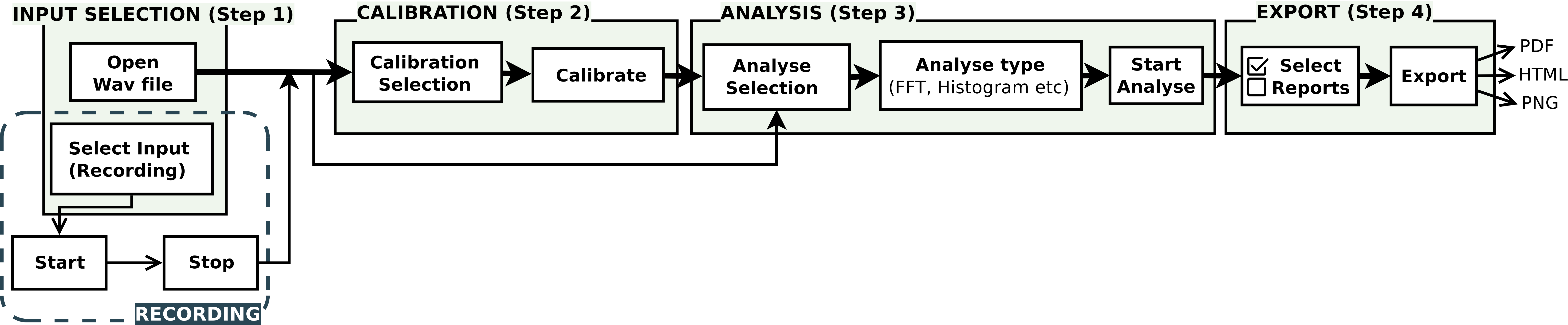
A standard workflow of the program usage can be broken down in the following four steps, as shown in figure 2.1.
2.1.1 Step 1: Select input
When starting the program a start dialog pops up. To open WAV files just drag
and drop them into the window or open them by clicking the ”Open WAV”
button.3
Afterwards the main program with the selected audio file(s) appears.
If you want to record audio click the ”Record...” button and a drop-down list with your audio
interface setup shows up. Select the desired channels to record and hit ”Confirm”. The
program is now ready to record. Start the recording with Menu ▸ Recording ▸ Record (or
ctrl+R). When finished stop the recording with Menu ▸ Recording ▸ Stop (or ctrl+S).
2.1.2 Step 2: Calibrate (optional)
For measurement purposes and to be able to plot the analyses with a dBSPL
scale4 ,
a calibration of the file is necessary. Nevertheless the calibration workflow stage is optional
and a qualitative analysis can be preformed without calibration, which results in a
dBFS5
scale. The calibration tone needs to be recorded in conformity with the standards with a 94dB 1kHz sound
source.6 .
To calibrate the channel change the drop-down list to ”Calib.”. Then mark the largest possible time
range containing the calibration signal by holding down the left mouse button and moving over the
waveform. Deselect by holding down the right mouse button. Finally click the ”Calibrate” button.
 (a) Drop-down
list
of
selections.
(a) Drop-down
list
of
selections.  (b) Selection
of
the
(calibration-)
waveform
with
currently
draging
the
deselection
(red
rectangle).
(b) Selection
of
the
(calibration-)
waveform
with
currently
draging
the
deselection
(red
rectangle).
| Figure 2.2: | Detailed explanation for calibration. |
2.1.3 Step 3: Analyse
To select the region to be analyzed, click and hold the left mouse button and mark an area of the waveform (green rectangles). To refine your selection, click and hold the right mouse button to deselect (red rectangle when active, see figure 2.2b). Subsequently select the type (FFT, Histogram, SPL etc) from the drop-down list and start the analyse by hitting the ”Analyse” button underneath. Your analyse (hereafter called analyze widget) appears now in the ”Analyzer” window, whereas the ”Editor” window still contains the waveforms and selections. By modifing the existing selection, your old analyze widget will be replaced. When you activate another selection (drop-down menu, figure 2.2a) the new analyze will be placed underneath the old one, which offers the possibility to compare different channels, time-regions or to store several analyse types of one region.
2.1.4 Step 4: Export
When all analyse widget parameters (time weight, frequency weight etc.) are set as you want them
to be exported, tick the ”Report” checkbox on the right of every widget. A shortcut for
(de-)selecting all widgets for export can be found under Menu ▸ Report ▸ Select all (or
ctrl+A).
With Menu ▸ Report ▸ Export... (or ctrl+E) the export file save dialog opens up and let you specify
where to save the report and which in format (PDF, PNG or HTML).
For detailed information please follow section 2.2.8.
2.2 User Manual
2.2.1 Data flow chart and layout
Figure 2.3 provides an overview of the main layout areas of SNARE and their naming, which is in detail the menu bar, the editor window with an opened track and its track control panel as well as the track navigation, the analyzer window with the analyze control panel and the status bar (from top). Whereas the data flow chart in figure 2.4 covers a coherent view on all functionalities accessible by the end-user.
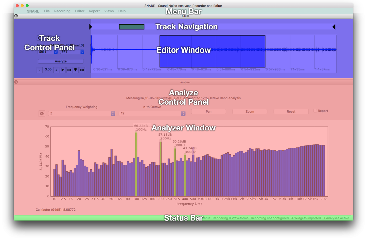
| Figure 2.3: | Layout overview of SNARE with an audio sample loaded from the high voltage corona discharge measurement series. (Details on the measurement see section 1.3.) |

2.2.2 Open file(s)
▸ctrl + O or drag & drop into window.
Beginning from the left, the user can record or open existing audio file(s). All common
RIFF WAVE files with 16bit or 24bit bit depth in 44.1kHz, 48kHz or 96kHz are readable.
When the file can’t be read, an error in the console is returned with detailed description, e.g. when the
file is corrupt. In the main window the function is accessible through the menu or the above mentioned
shortcut.
2.2.3 Recording
Select Input ▸ctrl + I
First the channels for recording from your build in or external audio interface need to be selected. This
can be done via start dialog’s ”Recording...” button or in the main window through Menu ▸ Recording
▸ Select Input... or the mentioned shortcut. The selected channels will be added in the Editor and are
ready for record.
Start ▸ctrl + R
To start recording go to Menu ▸ Recording ▸ Record or use the given shortcut. Due to buffer handling
the waveform will be updated every 10 seconds. The files are saved in the program main folder with
format: DD.MM.YYYY-hh.mm.ss__InterfaceName_[ChannelNo].wav. A time counter in the task bar
shows information depending the record.
Pause ▸ctrl + P
Pause the recording with Menu ▸ Recording ▸ Pause or the given shortcut. After the pause use Start
recording to continue.
Stop ▸ctrl + S
To finish the recording with Menu ▸ Recording ▸ Stop or the given shortcut. You can see a recording
counter in the task bar.
2.2.4 Channel functions (zoom, navigation, marker, play)
The following functions are all accessible through the track control panel.
To zoom use the ”+” and ”-” buttons. The current zoom status is represented in the track scroll bar
(see 2.2.10).
To navigate hold the shift key pressed, then click with left mouse button on the waveform
and hold it down while navigating through it. Alternatively make use of the track scroll
bar.
Double click in the waveform to position the cursor. After that you can either set a marker or play
or pause using the marker button  or the playback button
  of the Track Control Panel.
Alternatively you can use the ctrl + M shortcut for marker. To go to the next or previous marker use
the
of the Track Control Panel.
Alternatively you can use the ctrl + M shortcut for marker. To go to the next or previous marker use
the  and backward
  buttons.
2.2.5 Selection
Before analysing or calibrating a time range selection needs to be specified. To do so drag the mouse
over the waveform while holding down the left mouse key. This will draw a green selection rectangle
when active. Refine your selection by adding additional time ranges or remove parts of the selection by
holding down the right mouse key (red rectangle when active). The removing of a selection is pictured
in the QuickGuide figure 2.2b.
Complete new selections can be added by Menu ▸ Editor ▸ Add new selection.
2.2.6 Calibration
For calibration a 1kHz 94 dBSPL nominal sound pressure reference needs to be recorded on the same
channel that should be calibrated.
Switch to ”Calib.” selection in the drop-down list (initial value ”Sel 2”) as shown in figure 2.2a. Then
select the biggest possible range with the calibration signal and hit the ”Calibrate” button. All your
analysis are now calibrated and shown in dBSPL instead of dBFS. Calibrated analysis can
be distinguished from uncalibrated ones by the additional ”Cal factor” note under the
widget.
2.2.7 Analyze
When pressing the ”Analyze” button of the Track Control Panel the AnalyzeWidget will show up in the Analyzer window. When analyzing the same selection of the same track again, the old AnalyzeWidget will overwritten with the new selection. For new selections or tracks, a new AnalyzeWidget will be added to the Analyzer window. The user can choose between the following analysis through the analyze type selection or create own AnalyzeWidgets as explained in 2.2.11.
Octave band analysis (FFT)
Apply a one sided octave band analysis with the FFT algorithm with N = 1, 3, 6, 12, 24 on the selection. The values are plotted frequency-weighted depending on the widget selection.
Sound pressure level over time (SPL)
Plots the sound pressure level dBSPL over time of the current selection, the values are frequency- and time-weighted depending on the widget selection.
Histogram (Hist.)
The histogram analysis is a sound pressure level occurrence distribution. In other words the probability of occurrence of the SPL is plotted against the SPL values. Furthermore a cumulative sum curve is overlayed.
AnalyzeWidget
Control Panel Regarding the widget itself, the user can configure the widget parameters and plot
navigation through the Analyze Control Panel of each widget. This covers frequency weighting
(A, B, C, D, Z), time weighting (slow, fast, impulse) and optional parameters. As well as
zoom, pan (navigation) and reset functionality of the plot. To zoom in the plot, click the
zoom toggle button and drag a rectangle in the AnalyzeWidget plot. Navigate through
the plot by toggling the pan button. Zoom out by resetting the settings with the reset
button.
Labels On top of each widget is a title label that fulfills the format:
filename[channelNo] selectionNo: analyzeType
and on bottom of each widget is an modifiable info label with additional information e.g. whether
calibration is set:
Calibrated: no, calibration factor Weighting: A, B, C, Z Meter Speed: slow, fast, impulse.
2.2.8 Generate Report
To export a report file the identically named checkbox of all desired AnalyzeWidgets needs to be checked, which can be found rightmost on the Analyze Control Panel. All widgets can be activated by the shortcut ctrl + A or Menu ▸ Report ▸ Select all and deactivated by Menu ▸ Report ▸ Deselect all. When finished with the report selection, the report can be generated by ctrl + E or Menu ▸ Report ▸ Export... Set the save location and specify the file format in the dialog: PDF, HTML or PNG. For PDF every channel will be exported on a new page, whereby after every third widget a new page will be created. HTML will export all information among themselves and PNG will export the raw plot only without title and information label of all selected AnalyzeWidgets as Portable Network Graphics.
2.2.9 Views
Through Menu ▸ Views ▸ the layout of SNARE can be switched between nested view (which is set by default) or tab view. Second will group all analyses in one tab and the editor in the other tab. A quick switch between the view modes is accessible by ctrl + T for tab view or ctrl + N for nested view. In addition the modular Editor and Analyzer part of SNARE program can be dragged and dropped freely to be arranged to the users need.
2.2.10 Track Scrollbar
The Track scrollbar helps to orient oneself by showing the current zoom status represented by a green rectangle related to the longest file length figured as the whole bar. It can be used to scroll through the files simultaneously by click and drag the green rectangle.
2.2.11 Status Bar
The dynamic status bar provides information about the current calculation processes like Rendering or Recording. It also shows the among of imported widgets and the number of current active widgets.
2.2.12 Menu Bar
The menu bar offers access to the main functionality of SNARE. It is grouped in File, Recording,
Editor, Report, Views and Help and contains in detail:
File: Open Wav...
Recording: Select Input.., Start, Pause, Stop
Editor: Add new Selection
Report: Select all, Deselect all, Export...
Views: Tab View, Nested View
Help: QuickGuide and documentation.
2.3 Create own Analyze Widgets
Creating own widgets only works with an installed Python interpreter and the Python
scripts7 , it
does not work with the freezed binaries.
For a new Widget duplicate the example AnalyzeWidget folder to AnalyseTools/WidgetNAME and
adjust the ending of the containing files to *NAME, where NAME stands for the unique AnalyzeWidget
short name, e.g. ”Fft”. Make sure, the folder prefix is Widget*. Also adopt the class names
of the files (e.g. „WidgetExample.py“ contains the WidgetExample class) to coincident
the file name. Also ensure to correct the library imports in the header part of the scripts
to:
from AnalyzeTools.Widget.*NAME import …
A capsuled AnalyzeWidget consists of the necessary CalculationNAME.py, PlotNAME.py,
WidgetNAME.py and Info.txt files. Optional a NavNAME.py can be added, to extend and shadow the
existing NavMenuStandard class, e.g. for another dropdown selection when optional widget parameters
are set. After the Info.txt file is adopted as explained in 2.3.2, the widget is now ready and will be
dynamically imported into SNARE. Now its time to adopt the signal processing in the
CalculationNAME class to your needs.
2.3.1 Info.txt
The AnalyzeWidget Info.txt text file contains the basic widget parameters and needs to meet following
requirements and structure. It assigns variables in a table, where ident (variable names) are set
against the values (variable values), split by a colon separator. The first two rows are ignored, as well
as empty lines.
Needed variables are: ShortName, Filename.
Optional variables are: OptParameter1, OptParameter1InitVal, OptParameter2, OptParameter2InitVal,
OptParameter3, OptParameter3InitVal, ParameterFqWeightingInitVal, ParameterTimeWeightingInitVal.
2====Fill out the values under "ident: values" for your Widget====
3
4ident: values
5
6ShortName: FFT
7Filename: WidgetFft
8OptParameter1: nthfft
9OptParameter1InitVal: 3
10OptParameter2: None
11OptParameter2InitVal: None
12OptParameter3: None
13OptParameter3InitVal: None
| Listing 2.1: | Sample Info.txt file, containing one optional parameter. |
2.3.2 Analyze Control Panel adaptation
If the widget contains optional parameters, in the most cases these parameters should be controlled by the end-user. To realize this we, however need to customize the Analyze Control Panel, more precisely the Nav class. Normally a widget (like the example widget) takes the NavMenuStandard class from the AnalyzeTools/Nav.py file. To adopt the menu, you can have a look at the Fft widget, where the NavMenu class from the same file is derevated and adjusted. However, we need to proceed in this case by adding an additional NavNAME.py in the widget folder and adopt the import in the WidgetNAME class as well as adjust the initialization in the WidgetNAME constructor.
2.4 Editor Adjustment Tutorial
In this tutorial the design of the Editor-module will be examined in detail and it will be shown, how this design can be used to easily adjust the program behaviour to fit a specific purpose.
2.4.1 Advantages of Qt’s Signal/Slot
The Editor area consists of all classes that start with Track, most of which inherit from TrackManager. The design heavily relies on Qt’s Signal-Slot System. It allows the programmer to define a signal, that will be triggered on a certain event, a slot that matches the parameters of the signal and a connection between one signal and one or many slots. These connections can be made or broken at runtime. In the implementation of SNARE’s editor area, we defined a set of all required signals and slots in the base class, TrackAbstract and also automated the connection making. This means, if any class derived from TrackAbstract gets instantiated, the constructor will, if provided with an object-reference, automatically connect its signals and slots with the parent object’s signals and slots. The endpoint of those signal paths, the TrackManager also has the same interface, but could be seen as a kind of router for the signals. In the following tutorial, we will show how this property can be used to make adjustments to the editor area.
2.4.2 Code Example
In its default set-up, SNARE is configured to analyse a multi-track recording of one event, meaning that the time on all tracks is assumed to be identical. But one might also want to analyse a set of data containing different events on different tracks. In this scenario it would not make sense that the drawing of selection rectangles is synchronised on all tracks.
2 self.sender().slo_startSelection(QGraphicsSceneMouseEvent)
3
4 def slo_mouseRelease(self, QGraphicsSceneMouseEvent):
5 self.sender().slo_endSelection(QGraphicsSceneMouseEvent)
6
7 def slo_mouseMove(self, QGraphicsSceneMouseEvent):
8 self.sender().slo_moveSelection(QGraphicsSceneMouseEvent)
| Listing 2.2: | Separated channel selections |
2 self.slo_startSelection(QGraphicsSceneMouseEvent)
3
4 def slo_mouseRelease(self, QGraphicsSceneMouseEvent):
5 self.slo_endSelection(QGraphicsSceneMouseEvent)
6
7 def slo_mouseMove(self, QGraphicsSceneMouseEvent):
8 self.slo_moveSelection(QGraphicsSceneMouseEvent)
| Listing 2.3: | Synchronised channel selections |
The listing above shows the slots of the TrackManager that receive any mouse input from the QGraphicsScene. In the first version, the signal is sent back to the object that emitted the signal by calling the corresponding slot of that signal. (self.sender() returns the sending object) The second version shows how the signal can be sent back to all tracks by emitting the corresponding signal of the TrackManager. This works, because all track objects are subscribers to this signal of their parent object. (The alternative being a for-loop over all tracks, e.g. to handle one of the tracks differently)
Similar adjustments could be made to: synchronisig the displayed waveform-portion, placing markers and cursors, selection and analysis-type menu and others.
7 Appendix
7.1 Appendix A: Setup Tutorial for Windows
This tutorial will explain the necessary steps to install Python with all required libraries to run SNARE on Windows. These steps were tested using a new Windows 7 installation. Please note that all parts, Python and its libraries, are constantly developed and changed, therefore this procedure might not work with future versions.
7.1.1 Installing Python
SNARE has been developed with Python 3.4 and Python 3.5. We recommend using the latest version, Python 3.5, which can be obtained from the Python Project’s web page:
https://www.python.org/downloads/windows/
Select a stable release of Python 3.5 from the list and proceed to download. On installation, it is important to allow Python to add its directory to the windows PATH registry entry. This way Python can be accessed from any command line interface.

7.1.2 Installing the SciPy packages
The easiest way to install compatible packages for the SciPy environment is to download them from:
http://www.lfd.uci.edu/~gohlke/pythonlibs/
To run SNARE on a 32bit Windows, one will need:
- numpy-1.11.2+mkl-cp35-cp35m-win32.whl
- scipy-0.18.1-cp35-cp35m-win32.whl
To install, open a command line interface in the download directory and call:
pip install "numpy-1.11.2+mkl-cp35-cp35m-win32.whl"
pip install "scipy-0.18.1-cp35-cp35m-win32.whl"
7.1.3 Further packages
SNARE also requires some other packages that can be downloaded automatically by pip. Simply use:
pip install pyaudio
pip install pyqt5
pip install pandas
pip install matplotlib
7.1.4 Run SNARE
SNARE can now be easily launched by double-click on the ”Start.py” file or by calling it through a command line interface:
python Start.py